
For human, animal and plant whole-genome, exome and panel data: family, case–control and tumour–normal designs. We follow GATK Best Practices and write every filter parameter into the report.
| You provide | You receive |
|---|---|
| fastq or bam files | QC and coverage report |
| Sample sheet: pedigree, phenotype, pairing | VCF plus annotated variant tables (Excel) |
| Reference genome version (hg38/hg19 or other species) | Candidate variant tables and figures |
| Target bed file (WES / panel) | Code, parameters and methods paragraph |
Typical turnaround: 7–12 working days for the standard scope; complex designs as stated in the written analysis plan. Quotes are per project, returned within 1 working day.
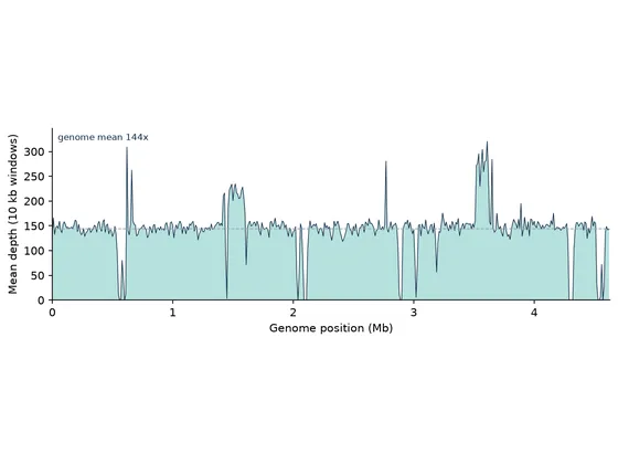
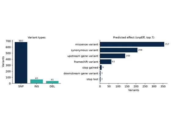
Joint calling works from 2 samples; more samples make low-frequency filtering more stable. Single samples are fine too, and the report explains the difference.
Our deliverables are for research use. Clinical interpretation must be done by an accredited laboratory.
Yes. Exome-based CNV calling is less precise than WGS and the report includes a confidence statement.
For animal, plant, microbial and human cohorts from resequencing or array data: population structure, selection signals, trait association, domestication and evolutionary history.
| You provide | You receive |
|---|---|
| fastq, bam or VCF files | High-quality SNP set (VCF) with statistics |
| Sample sheet: population, phenotype, geography | Publication-ready figures for structure, selection and GWAS |
| Reference genome and annotation | Candidate region and gene tables |
Typical turnaround: 15–25 working days for the standard scope; complex designs as stated in the written analysis plan. Quotes are per project, returned within 1 working day.
No public example is available for this analysis yet. Deliverables follow the same structure as our sample reports (report, figures, tables, code, methods text); the specific figures are listed in the written plan.
It depends on heritability and effect size; there is no single answer. At the plan stage we state the effect range detectable with your sample size.
Mixed linear models correct for structure and relatedness; the report includes QQ plots and inflation factors as evidence.
For gut, soil, water, clinical and other microbial community studies. Amplicons suit composition comparisons; shotgun metagenomics suits function and fine taxonomy. We explain the difference at the plan stage.
| You provide | You receive |
|---|---|
| fastq files and primer information (amplicons) | ASV / taxon abundance and annotation tables |
| Sample sheet: groups, sampling time, clinical or environmental variables | Publication-ready diversity, composition and differential figures |
| Host genome for host removal, if applicable | Functional annotation and pathway difference tables |
Typical turnaround: 10–15 working days for the standard scope; complex designs as stated in the written analysis plan. Quotes are per project, returned within 1 working day.
No public example is available for this analysis yet. Deliverables follow the same structure as our sample reports (report, figures, tables, code, methods text); the specific figures are listed in the written plan.
16S routinely resolves to genus; species-level labels need caution. For species or strain resolution we recommend shotgun metagenomics and say so in the plan.
We rarefy according to the data distribution or use rarefaction-free methods, and include rarefaction curves in the report.
For histone marks, transcription factor binding, chromatin accessibility and DNA methylation (WGBS / RRBS / 850K arrays). The focus is linking epigenetic signal to gene expression and regulatory elements.
| You provide | You receive |
|---|---|
| fastq files including input / IgG controls (ChIP) | QC and peak-calling statistics |
| Sample sheet: antibody, treatment, replicates | Peak files (bed / bigWig) and annotation tables |
| Reference genome version | Publication-ready differential region and motif figures |
Typical turnaround: 10–15 working days for the standard scope; complex designs as stated in the written analysis plan. Quotes are per project, returned within 1 working day.
No public example is available for this analysis yet. Deliverables follow the same structure as our sample reports (report, figures, tables, code, methods text); the specific figures are listed in the written plan.
Peaks can be called, but the false-positive risk rises; the report says so and recommends adding a control.
With IDR and inter-replicate correlation, plus per-sample TSS enrichment scores as quality evidence.
Tell us the data type and the question you want answered. You will receive a written analysis plan and quote within 1 working day.
Request an analysis plan